Jim Williams
In January/February 2013, Jim Williams wrote to Stuart Anderson;

Steven Strogatz (left) and Jim Williams (right) - high school classmates
"Hi Stuart,
I have been fascinated by the problem of subdividing a square into smaller squares each of different size since I read Martin Gardner’s book as a child. A couple weeks ago I decided to write a program to search for perfect squares. This was for my own amusement as I didn’t much expect anyone else would be interested.
However I found your web site, squaring.net, and figured I would share the list I found in case you were interested in posting it. There’s a lot on my list not currently in your posted downloads."
"... I am surprised with all the thought that seems to have gone into this problem that no one has tried what I did before. Mostly it is FAST versus SMART. I was able to process about 10^8 trials per second with a success rate ranging from 1 in 10^8 to 1 in 10^9. (with the help of a XEON 5500 CPU)."
"The basic idea is to take the electrical network associated with a square and split it roughly in half by cutting exactly three nodes. This seems to be possible for most (but not all) low order squares, and probably close to half of squares up to order 33. The outer loops create a large library of “half networks” and the inner loop attempts to pair up two halves to form a perfect square. While this doesn’t reduce the search space, by moving most of the computation to the outer loops, the inner loop can run extremely fast.
It would be interesting if it could be proven that the electrical network (or its dual) for any perfect square of up to order X can be cut approximately in half with the larger half containing no more than Y% of total edges but cutting at most Z nodes, and find numbers for X, Y, and Z. This looks hard and the resulting value of Z might be too large to be interesting, but if possible could allow enumerating all perfect squares up to a bigger number."
Jim had produced over 2.8 million perfect squared squares in the couple of weeks over Xmas and New Year. After 6 weeks of running his program Jim produced over 15 million perfect squared squares. No new squared squares were found in the order 20's, but the majority of the squares, those being in order 30's and 40's were nearly all new discoveries.
Jim Williams Perfect Squared Square Discoveries
- 9189 Order 30 SPSSs, (600k), 2140 Order 30 CPSS isomers
- 26961 Order 31 SPSSs, (1.4M), 7208 Order 31 CPSS isomers
- 62835 Order 32 SPSSs, (3.4M), 20108 Order 32 CPSS isomers
- 142880 Order 33 SPSSs, (8.2M), 7016 Order 33 CPSS isomers
- 9922 Order 34 SPSSs , (600k), 4 Order 34 CPSS isomers
- 21852 Order 35 SPSSs, (1.4M), 13 Order 35 CPSS isomers
- 47028 Order 36 SPSSs, (3M), 27 Order 36 CPSS isomers
- 99746 Order 37 SPSSs, (7M), 53 Order 37 CPSS isomers
- 205562 Order 38 SPSSs, (15M), 102 Order 38 CPSS isomers
- 414126 Order 39 SPSSs, (32M), 182 Order 39 CPSS isomers
- 802970 Order 40 SPSSs (64M), 377 Order 40 CPSS isomers
- 1506178 Order 41 SPSSs (123M), 604 Order 41 CPSS isomers
- 2662359 Order 42 SPSSs (226M), 1093 Order 42 CPSS isomers
- 4241399 Order 43 SPSSs (372M), 1679 Order 43 CPSS isomers
- 5099311 Order 44 SPSSs (464M), 1899 Order 44 CPSS isomers
- Total SPSSs; 15352318 Total CPSS isomers; 42505
Jim William's method has led to a huge increase in the number of known SPSSs. Prior to his work only tens of thousands were known, now there are millions in the catalogue. With so many to examine, it is possible to look for rare exceptions and test many conjectures regarding the characteristics and composition of simple perfect squared squares. For example, there are only 24 simple perfect squared squares and only 1 compound perfect squared square to be found with a side less than 200. There were none found in orders 28 or 29, it started to look like they had all been found in the lower orders. Then Jim found 2 SPSSs with sides of 185 and 199 in order 32. The Bouwkampcodes are;
32 185 185 (80,51,54)(29,19,3)(16,41)(10,25)(35,26,43,15)(28,20,33)(9,17)(36,8)(7,13)(1,6)(30,62,5)(57)(34,2)(32)
32 199 199 (89,46,64)(28,18)(23,59)(15,13)(36)(33,37,34)(29,4)(21,32,76)(25,16)(9,7)(10,11)(2,5)(48,17)(14,1)(44)(31)
Many of the exceptional examples of 'Special Squared Squares', that is, Perfect Squares with unusual or extreme properties, are taken from Jim William's collection.
Jim Williams 2014 CPSS and SPSS Discoveries.
Jim Williams has in 2014 completed a major enumeration of Compound Perfect Squared Squares (CPSSs) orders 33 to 36 and Simple Perfect Squared Squares (SPSSs) order 33.
Jim Williams Software.
Jim made available the software which he developed for finding perfect squared squares in 2013 and 2014. See the downloads page for source code.
Jim has also provided a more detailed explanation of the 2013 algorithm;
2013 Algorithm Summary
Attached is the output from my previous run which just completed after about six weeks of computing. The goal was to find as many perfect squares as possible in a practical amount of time. No particular effort was made to search for a particular kind of square ( low order, etc. ) but rather just to find the most.
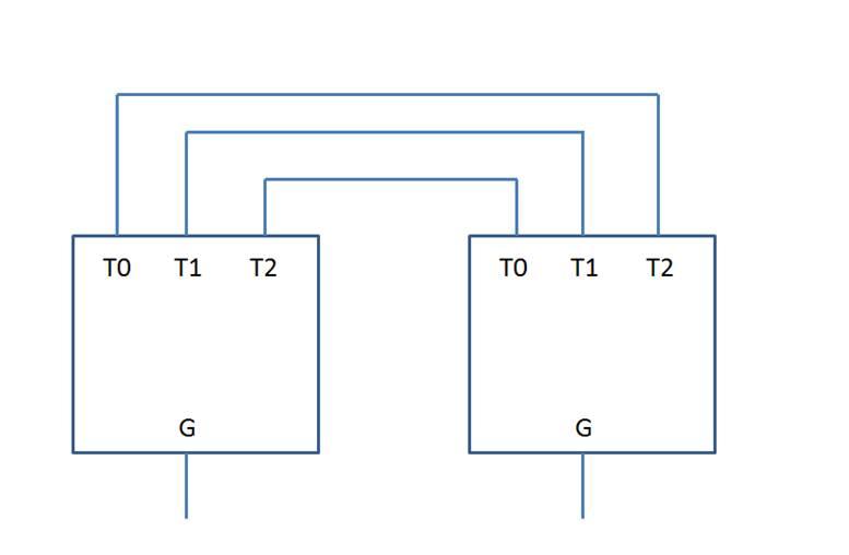
The algorithm looks for squares for which the associated electrical network can be cut roughly in half but cutting exactly three nodes. The resulting two halves are connected together as follows.
Each network is a 4-terminal network with terminals being ground, T0, T1, and T2. The combined network is as shown with the two grounds being the two poles. If the resistance between these two is exactly one, then corresponding rectangle is a square.
The half-networks are divided into two types (sexes) arbitrarily denoted as type M and type F. Type F networks are planar networks with at least 3 connections to each internal node, and at least two connections to each external node (G, T0, T1, and T2). Type M networks are similar except that terminals T0, T1, and T2 must have a minimum of one connection, and none the nodes T0, T1, or T2 may connect to any of the others. The result is that when a type M network is connected to a type F network, each of the connection nodes will have a minimum of 3 connections and there will be no parallel edges created.
Each type F network can be converted to a reference graph by adding one addition node (the reference node) and 4 additional edges, one from the reference node to each of the terminal nodes. Reversing this process, all type-F networks can be generated by generating the set of all 2-connected degree-3 planar graphs, then selecting any node with exactly 4 edges as a reference node and removing that node and its edges, and using the nodes which used to connect to the reference node as the terminals.
Each type-M network can be converted to a type-F by adding one edge from T0 to T1 and adding a second edge from T1 to T1. Conversely all type-M networks can be created by selecting a type-F network with the following properties and removing the connection from T0 to T1 and T1 to T2. The properties are:
1. There is a connection from T0 to T1
2. There is a connection from T1 to T2
3. There is NOT a connection from T0 to T2
4. There are at least three connections to T1
After creating a list of all type-M and type-F networks of up to a given size, these networks are pre-screened. If any internal resistor has current with is identically zero regardless of the terminal voltages, or if it has two resistors whose current is identically equal independent of the terminal voltages, then the network is excluded. A reasonable percentage of the networks can be excluded this way.
For selecting pairs of networks it would be very useful if we could characterize the effective resistance of the network in a single number, R. If we could do this, then it would remain only to search for potential mates with resistance (1-R) such that the pair would have a resistance of exactly one, and form a square. Unfortunately it is not possible to characterize the resistance of a 4-terminal number with a single value. However it can be approximated. Specifically I used two approximations called Rmin and Rmax. Rmin is the result of shorting together the terminals T0, T1, and T2, and measuring the resistance from this shorted terminal to ground. Rmax is the result of forcing an equal current through each of T0, T1, and T2 and calculating the ratio of the average voltage of the three to the total current of the three. Amazingly when two networks are connected, the resistance of the combined network (measured between the two respective grounds) is always greater than the sum of the Rmin’s and less than the sum of the Rmax’s.
Using Rmin and Rmax in this way allows a quick way to screen potential mates to see if they might form a square. Across the general set of type-M and type-F networks, this screen if about 75% effective. Only about 25% percent of pairs pass this. However for this run I filtered on the difference between Rmax and Rmin. In particular I generated all type-M and type-F networks up to order 22, but added to the library only those networks for which Rmax – Rmin < 0.01. This somewhat limits the search space, but increased the number of perfect squares found per unit compute time by a factor of 10. Geometrically this results in the squares that not only can be divided in half by three line segments connected by two jogs, but the lengths of the segments are about the same and the jogs will be small (relative to the more general case).
The resistance of the 4-terminal network can be exactly characterized by a symmetric 3x3 resistance matrix. If the resistance matrices for the two half-networks are R1 and R2, then the resistance of the combined network can be calculated by solving the following matrix equation: (R1 + R2) * I = ( 1, 1, 1). “I” will be the 3 element current vector indicating the current through each of the connections when one volt is applied between the respective grounds. If these three elements sum to one, then the combined network represents a square.
To evaluate whether a pair of networks forms a perfect square, the following 4 tests are run in order.
1. Verify that sum of Rmin’s is less than 1 and sum of Rmax’s is greater than 1.
2. Solve 3x3 matrix equation to verify that resistance of combined network is exactly 1.
3. Verify that each of the three components of the “I” vector is unequal to the other two.
4. Generate combined network, solve for all components resistors, and verify that all currents are non-zero and unequal.
Test 1 can be run very quickly. All type-M networks are sorted into blocks of roughly equal values of Rmax. Within each block they are sorted in order of Rmin. Then for each type-F network a binary search can be done to locate all potential mates.
Test 2 is the critical performance path. The 3x3 resistance matrix for each half-network is pre-computed (off the critical performance path) so when evaluating the pair we have the values of R1 and R2. Solving the equation “(R1 + R2) * I = ( 1, 1, 1)” requires about 30 floating point operations and for speed all the loops have been unrolled. This equation is solved twice for each pair, once for the normal connection as shown above ( T0 ó T2, T1 ó T1, and T2 ó T0 ) and once for the reflected connection ( T0 ó T0, T1 ó T1, and T2 ó T2 ).
Test 3 is non-obvious. It is not a necessary condition that the three current components be unequal. However for perfect squares they almost always are and this test filters out about 99.9% of the cases passing test 2. Eliminating this test would causes all these to fall through to test 4 which would significantly slow down the square production rate.
Test 4 is the definitive test that determines whether a network is in fact a perfect square, however it is quite slow compared to the other tests so we need to screen out as many networks as possible before getting to test 4.
Some very approximate metrics of the run are as follows:
Total number of half-networks: 10^8 each of type-M and type-F
Total number of possible pairs: 10^16
Percentage of pairs passing test 1 2%
Of those percentage passing test 2 0.1%
Of those percentage passing test 3 0.1%
Of those percentage passing test 4 10%
Total perfect squares found 1.5*10^7
Run time 4*10^6 seconds (6 weeks)
Throughput (test 2) 10^8 tests per second
Jim Williams, February 2013
Jim Williams post 2014 enumeration of SPSSs and CPSSs
In April 2014, Jim used software he had written to enumerate complete orders of CPSSs. He was able to enumerate the known CPSS classes and isomers from order 24 to order 32, confirming the existing results, and to go further by extending the complete enumeration of classes of CPSSs and isomers from order 33 up to order 36.
| CPSS orders | CPSSs o33 | CPSSs o34 | CPSSs o35 | CPSSs o36 | Complete CPSS class totals |
22413 | 62273 | 172330 | 466508 |
| Complete CPSS isomer totals |
150669 | 429458 | 1206181 | 3337989 |
2014 May June ; With new software Jim enumerated the SPSSs of order 33. In 2 weeks he found all 378197 SPSSs of this order.
2016 April ; Enumerated the SPSSs of order 34 and 35. He found 990981 SPSSs in order 34 and 2578081 SPSSs in order 35.
2018 August ; Jim finalised the enumeration of CPSS orders 37, 38 and 39, including the isomers of each.
| CPSS orders | CPSSs o37 | CPSSs o38 | CPSSs o39 | Complete CPSS class totals |
1239742 | 3257378 | 8430928 |
| Complete CPSS isomer totals |
8961794 | 23989218 | 62894424 |
2020 July ; Jim enumerated the SPSSs of order 36 and 37. He found 6674067 SPSSs in order 36 and 17086918 SPSSs in order 37.
Updated 8th August 2020.